\begin{frame}
  \frametitle{The Definite Integral}

  \begin{block}{}
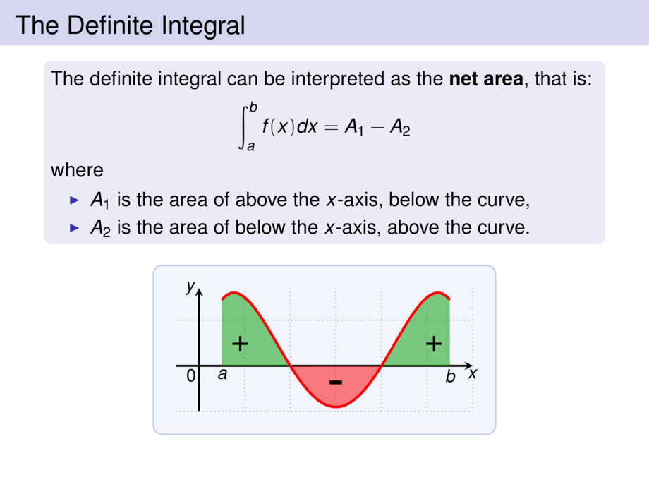
    The definite integral can be interpreted as the \emph{net area}, that is:
    \begin{talign}
      \int_a^b f(x) dx = A_1 - A_2
    \end{talign}
    where 
    \begin{itemize}
      \item $A_1$ is the area of above the $x$-axis, below the curve,
      \item $A_2$ is the area of below the $x$-axis, above the curve.
    \end{itemize}
  \end{block}
  \medskip
  
  \begin{center}
  \scalebox{.9}{
  \begin{tikzpicture}[default]
    \def\mfun{(-.9 + (\x-3+\mfunshift)^2 - .1*(\x-3+\mfunshift)^4)}

    \diagram[1]{-.5}{6}{-1}{1.7}{1}
    \diagramannotatez
    \def\mfunshift{0}
    \begin{scope}[ultra thick]
      \draw[fill=cgreen,draw=none,opacity=.5] plot[smooth,domain=.5:2,samples=100] (\x,{\mfun}) -- (.5,0) -- cycle;
      \draw[fill=cred,draw=none,opacity=.5] plot[smooth,domain=2:4,samples=100] (\x,{\mfun}) -- cycle;
      \draw[fill=cgreen,draw=none,opacity=.5] plot[smooth,domain=4:5.5,samples=100] (\x,{\mfun}) -- (5.5,0) -- cycle;
      \draw[cred] plot[smooth,domain=.5:5.5,samples=100] (\x,{\mfun});
      \node[anchor=north] at (.5,0) {$a$};
      \node[anchor=north] at (5.5,0) {$b$};
      \node[scale=1.8] at (.9,.5) {+};
      \node[scale=1.8] at (5.15,.5) {+};
      \node[scale=3] at (3,-.5) {-};
    \end{scope}
  \end{tikzpicture}
  }
  \end{center}
  \vspace{10cm}
\end{frame}