

19/50
\begin{frame}
\frametitle{Newton's Method}
\begin{center}
\scalebox{.8}{
\begin{tikzpicture}[default,baseline=1cm]
\diagram{-.5}{4}{-.5}{4}{1}
\diagramannotatez
\begin{scope}[ultra thick]
\draw[cgreen,ultra thick] plot[smooth,domain=-0:3.3,samples=200] function{-.5 + (.5*x)**3};
\node[include=cgreen] (r) at (1.58,0) {};
\node[anchor=south east] at (r) {$r$};
\end{scope}
\draw[gray] (3.2,-.2) -- node[at start,below,black] {$x_1$} node[include=cred,at end] {} (3.2,{-.5 + (.5*3.2)^3});
\tangent{4cm}{.5cm}{-.5 + (.5*\x)^3}{3.2}
\draw[gray] (2.28,-.2) -- node[at start,below,xshift=1mm,black] {$x_2$} (2.28,.2);
\end{tikzpicture}
}
\end{center}
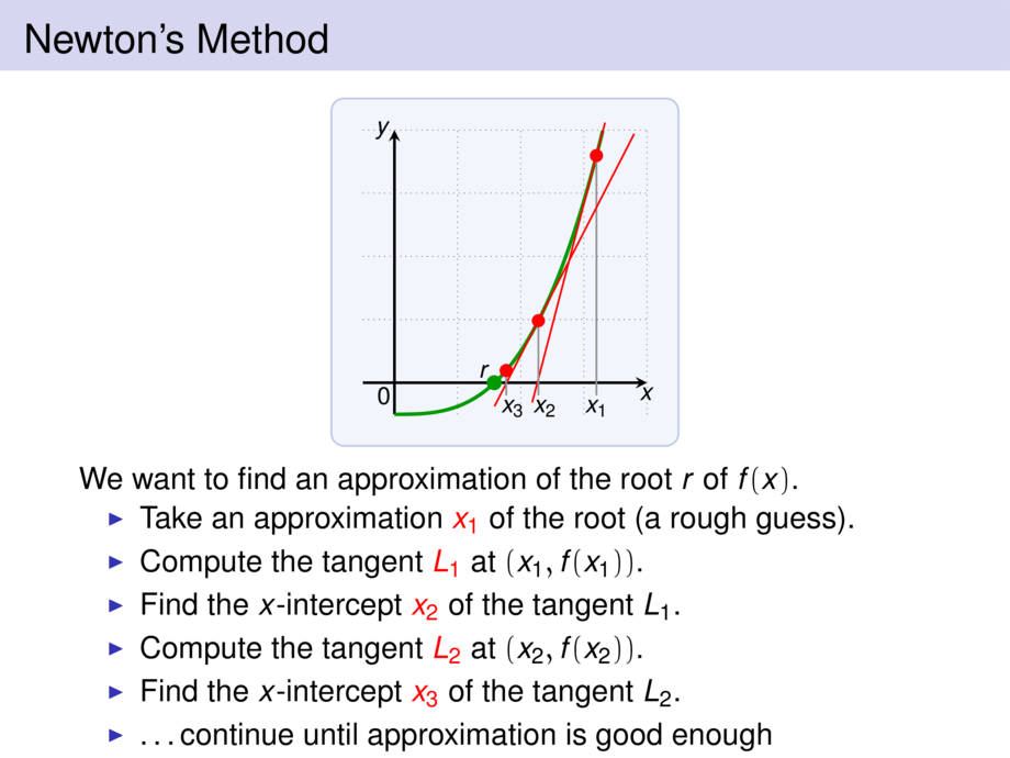
How can we compute $x_2$? \pause The tangent at $(x_1,f(x_1))$ is
\begin{talign}
y = \mpause[1]{f(x_1) + f'(x_1)(x-x_1) }
\end{talign}
\pause\pause
For the $x$-intercept $x_2$ of the tangent, we have:
\begin{talign}
0 = f(x_1) + f'(x_1)(x_2-x_1) \mpause[1]{ \implies \alert{x_2 = x_1 - \frac{f(x_1)}{f'(x_1)}}}
\end{talign}
\pause\pause
We can repeat this process to get $x_3$, $x_4$, $x_5$\ldots
\vspace{10cm}
\end{frame}